ADEL-Wheat (Architectural model of DEvelopment based on L-systems) is designed for
simulating the 3D architectural development of the shoots of wheat plants. The model has been
coupled with a light model adapted to field conditions (Caribu model), in order to allow calculating the
light interception by individual phytoelements during the crop cycle. Applications of such a tool range from the
interpretation of remote-sensing signals, to the estimation of crop light use efficiency, or to the
assistance in the ecophysiological analysis of plant response to light conditions.
The model is based on an analysis of developmental and geometrical similarities that exist among phytomers, to allow a
concise parameterization. Parameterising the model requires using experimental data to document a set of inputs described below.
Beside these user inputs, Adel also make use of constants and of relations (set and ‘readable’ in Adel.R, but not documented)
describing coordination of leaves, dynamics of geometry, computation of visibility and progression of senescence as a function of ssi.
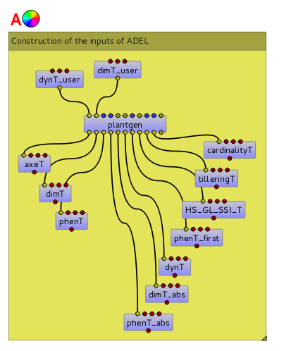
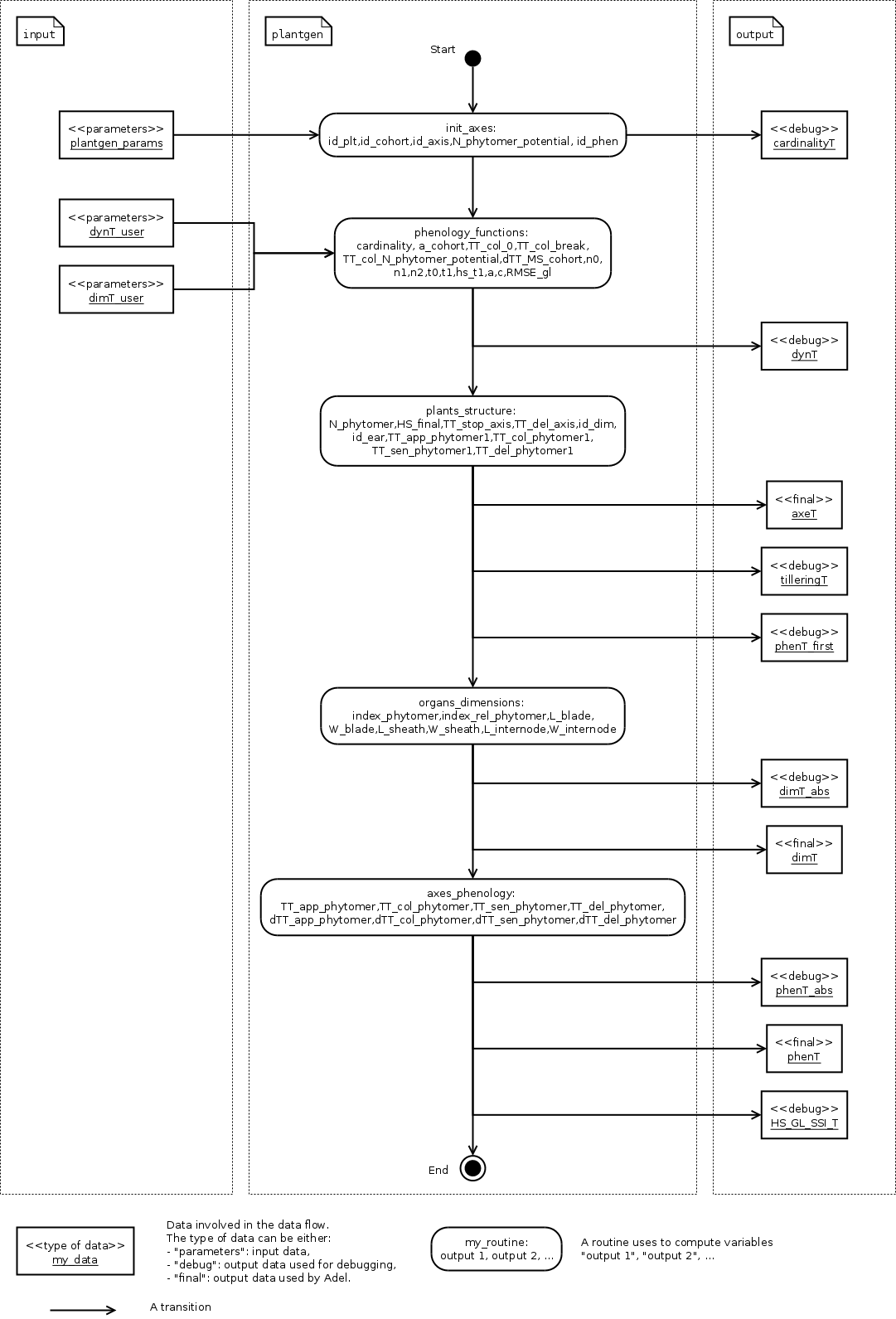
See Robert et al (Functional Plant Biology 2008) for description. The next figure
shows the global dataflow of Adel:
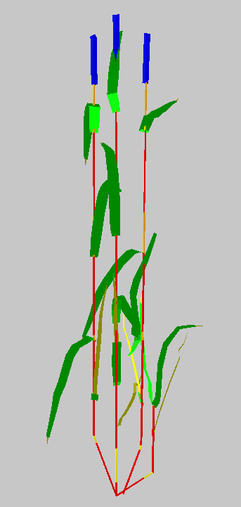
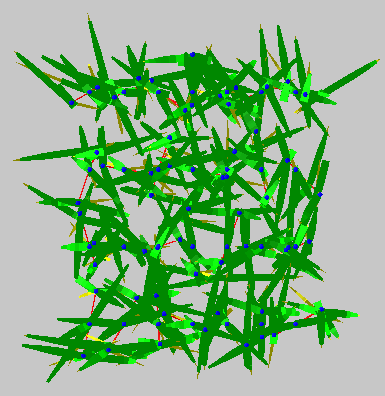
Simulations are visually realistic. And the model was shown to correctly reproduce important agronomic features such as kinetics of LAI and of plant height.
The following table presents simulation of Soissons variety with nitrogen fertilization:
Adel requires three kinds of inputs to be provided by the user:
inputs characterizing the development of plants in the canopy (topology, developmental rate and size of plants)
inputs characterizing the geometry of axes and of leaves
inputs characterizing the simulation (time step..) and the plot configuration (number of plants, position)
Units and conventions
- Dimension are expressed in cm
- Thermal time is expressed in °CD
Position of a phytomer on an axis: Most often (as described below) phytomer position in Adel are counted acropetally and are normalized relatively to the total number of phytomers
(leaf 1 relative position is 1/nf and flag leaf relative position is 1). Use of relative positions was chosen to allow sharing data between axes differing by the total number of phytomers
In later versions of Adel the relative phytomer number should be changed by the absolute one. With the convention that 1 is referring to the first true leaf.
Development is parameterized in a Rlist containing 3 tables (axeT, dimT and phenT).
These tables have dependencies (cross references). However some may be compatible with others if cross references are maintained. This allows for recombination of parameters.
axeT is the master table that organizes how each plant is described.
For each plant, the table contains a few explicit parameters that describe the phenology and the number of modules (eg time of appearance, number of axes and number of leaves on axes)
and identifiers that refer to information given in the other tables (dimT, phenT, earT).
All plants to be used for the reconstruction must be listed in axeT. If only one plant is given, Adel will clone that plant.
To have a correct simulation of tiller dynamics at the plot level, a minimum of 30 plants is recommended.
There is one line per axis. Columns are :
Column
Description
id_plt
Number (int) identifying the plant to which the axe belongs
id_cohort
Number (int) identifying the cohort to which the axe belongs
id_axis
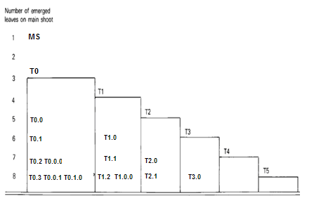
Identifier of the botanical position of the axis on the plant. “MS” refers
to the main stem, “T0”, “T1”, “T2”,…, refers to the primary tillers, “T0.0”,
“T0.1”, “T0.2”,…, refers to the secondary tillers of the primary tiller “T0”, and
“T0.0.0”, “T0.0.1”, “T0.0.2”,…, refers to the tertiary tillers of the secondary
tiller “T0.0”. See Botanical position of the axis on the plant..
N_phytomer_potential
The potential total number of vegetative phytomers formed on the axis. N_phytomer_potential
does NOT take account of the regression of some axes.
N_phytomer
The effective total number of vegetative phytomers formed on the axis. N_phytomer
does take account of the regression of some axes.
HS_final
The Haun Stage at the end of growth of the axis.
TT_stop_axis
If the axis dyes: thermal time (since crop emergence) of end of growth. If the axis grows up to flowering: NA
TT_del_axe
If the axis dyes: thermal time (since crop emergence) of disappearance. If the axis grows up to flowering: NA
id_dim
key (int) linking to dimT. id_dim allows referring to the data that describe the dimensions of the phytomers of the axis
id_phen
key (int) linking to phenT. id_phen allows referring to the data that describe the phenology of the axis
id_ear
Key (int) linking to earT. id_ear allows referring to the data that describe the ear of the axis.
For the regressive axes, id_ear=NA. For the non-regressive axes, id_ear=1.
TT_em_phytomer1
Thermal time (relative to canopy appearance) of tip appearance of the first true leaf (not coleoptile or prophyll)
TT_col_phytomer1
Thermal time (relative to canopy appearance) of collar appearance of the first true leaf
TT_sen_phytomer1
Thermal time (relative to canopy appearance) of full senescence of the first true leaf (this is : thermal time when SSI= 1)
TT_del_phytomer1
Thermal time (relative to canopy appearance) of disappearance of the first true leaf
dimT allows to describe a number of profiles of dimension, each profile
being associated to a value of id_dim. Dimensions of organs must be given for each
of the id_dim mentioned in axeT.
Positions on an axis are expressed as relative position (index_rel_phytomer = phytomer rank/N_phytomer);
Use of relative position makes it possible to use a same profile of dimension for axes differing in the final number of phytomers (N_phytomer);
Use of relative position makes it possible to document a profile with only some the phytomers on an axis:
Missing data will be estimated by linear interpolation according to index_rel_phytomer;
Actual dimension of the blade, sheath and internode of an axis are hence calculated according to id_dim and N_phytomer.
There is one line per phytomer documented.
Columns are :
Column
Description
id_dim
the identifier referred to in axeT. By convention, if the current id_dim
ends by 0 (e.g. id_dim=1110), then the current line documents
the dimensions of a regressive axis. If the current id_dim ends by
1 (e.g. id_dim=1111), then the current line documents the
dimensions of a non-regressive axis.
index_rel_phytomer
The relative phytomer position : index_rel_phytomer = phytomer rank/N_phytomer
L_blade
length of the mature blade (cm)
W_blade
Maximum width of the mature leaf blade (cm)
L_sheath
Length of a mature sheath (cm)
W_sheath
Diameter of the stem or pseudo stem at the level of sheath (cm)
phenT controls the dynamics of leaf appearance, ligulation, senescence and disappearance.
Internal rules of Adel coordinate sheaths and internodes to the blades so that phenT
controls indirectly the whole dynamics of plant development.
Positions on an axis are expressed as relative positions.
One timing of development has to be documented for each value taken by id_phen in axeT; axes sharing a same value of id_phen will share the same timing;
Use of relative position makes it possible to use a same developmental timing for axes differing in the final number of phytomers;
Use of relative position makes it possible to document a developmental timing with a number of value higher than the number of phytomers on an axis:
this is required because the dynamics of SSI shows a complex behavior(see below)
Timing of developmental events on a leaf is given relative to the timing of the event on leaf 1 of the axis;
Actual timing is computed from phenT and the data concerning leaf 1 in axeT.
For each id_phen, there is one line per value of index_rel_phytomer documented. For a smooth description of the
dynamics of SSI from crop appearance to maturity, approximately 40 values of index_rel_phytomer should be documented (for each value of id_phen).
More over for each value of id_phen, one line should be documented for index_rel_phytomer = 0, so as to allow interpolation.
Adel considers two categories of phytomers for describing the progression of senescence in leaf blades.
for lower leaves, the senescence progresses linearly as function of SSI and blades sequentially: the senescence of blade at rank n starts when senescence of blade n-1 has finished.
This means that the senesced fraction of leaf n is : 1+SSI -n. It depends only in ssi and there is no need for additional parameters.
for upper leaves, the progress of senescence is more complex and several leaf blades senesce simultaneously:
SSi2senT contains data to calculate the fraction of senesced area of each upper leaves as function of ssi.
The upper leaves correspond approximately to the leaves beard by an elongated internode.
The number of lower leaves showing a linear progress of senescence is called Nsenlow;
The number of upper leaves showing a complex progress is called Nsenup
All upper leaf blades start to senesce at the same time, that is at
;
Senescence of each upper leaf blade progresses first at a slow rate,identical for all leaves, then at a fast rate.
The parameter used to describe these kinetics are the value of the slow rate (R_sen1), the value of ssi (dssit1) at the onset of fast senescence
and the value of SSI (dssit2) at full senescence for each upper leaf.
The table defines the parameter values for the upper leaves.
There is one line per upper leaf and the number of lines of the file must be Nsenup
The values d_SSIt1 and dssit2 are specified in term of difference with the ssi at onset of upper leaves senecence (Nsenlow)
It should be noted that the present description of progress of senescence is over-parameterized, resulting in a constraint between parameters value.
This comes from the fact that at any time the sum of the rate of progress of senescence for all leaves should be one.
Complying with this constraint is not straightforward. So a user that do not know precisely the value of parameters in his experiment should probably use the default values to ensure a consistent behavior.
Column
Description
N_senup
Number of leaves that show two phases during senescence (the value is repeated for all lines!)
R_sen1
Rate of progress of senescence during phase 1 (the value is repeated for all lines !)
dssit1
(SSI when the leaf blade starts phase 2) - Nsenlow)
dssit2
(SSI when the leaf blade is 100% senesced - Nsenlow)
Input are required to define the geometry of leaves (normalized 2D shape, midrib curvature and azimuth) and the geometry of stems (inclination, azimuth)
Normalized 2D shapes are leaf width variations with distance to the base of the leaf, both axes being normalized so that max values is 1.
Normalized 2D shapes and midrib curvature are stored as collections and Adel will draw and individual leaf by scaling a 2D shape plus taking a midrib curvature from these collections.
The inclination of axes is defined by two parameters DredT and Tillerinc.
DredT represents the horizontal distance between the main stem and a tiller at flowering.
Tillerinc represents the angle of insertion of a tiller at flowering.
When a tiller grows, it starts with angle of 3° compared to the vertical. Then, during the period of extension of the lower internode, insertion angle increases up to the value Tillerinc.
It will keep this value until the top of the stem reaches the distance DredT from the main stem. When this is reach,
the two upper visible nodes rotate so that the top of the tillers remains at distance DredT. Any internode that elongate
later is vertical. Note that when sheath disappear, new node become visible and will become involved in the process.
genGoeaxe (see below) includes a parameter to randomly tilt the main stem of a small value around the vertical. When the main stem is tilted, all the plant follows
The collections for 2D leaf shape and for leaf curvature should be specified as one list of lists of matrices for 2D shape and one list of matrices for midrib curvature.
the first level in the list is for collection index
the second level is for matrix index.
See alea for more information.
Besides these collections, R functions should be provided as inputs. A first list of function is for defining the axis geometry;
A second list of functions is for selecting shapes in the collections mentioned above.
The first list should provide 3 R functions of axis number (0 = main stem) that return:
azT : the azimuth(deg) of the first leaf of the axis with reference to the azimuth of the parent axes
incT : the inclination (deg) of the base of the tiller compared with main stem
dredT : the distance (at maturity) between tiller and main stem
These functions can be generated by the predefined genGeoAxe node or be freely user-defined in a freeGeoAxe node.
In genGeoAxe
The azimuth of a tiller stem is the same as that of the axilling main stem leaf.
The azimuth of the first leaf of a primary tiller is with an angle of 75° relatively to that of the axilling main stem leaf.
For secondary tillers, the azimuth of the first leaf is also with a fixed angle relatively to that of the parent tiller.
The second list should provide two Rfunctions for drawing in the collections of leaf shape
Inputs have to be axis number, leaf position, leaf position counted from top, and leaf stage, defined as current length/final length.
Returned values have to be :
azim : the azimuth (deg) of the leaf compared to the previous one
Lindex : the index of the collection to use for leaf curvature
These functions can be generated by the predefined genGeoLeaf node or be freely user-defined in a freeGeoLeaf node:
Time step is given as a list of values of thermal times for which a mock-up is to be produced.
Positions of plants within the plot are given externally from adel to a planter.
The thermal time of leaf tip appearance and leaf collar appearance given in phenT are used to calculate a number of features;
- the leaf extension (blade + sheath) is simulated as starting 0,4 phyllochron between tip appearance, and having a constant rate (cm.°C-1.J-1) for a duration of 2 phyllochrons
- The model calculate the length of the hidden part of a leaf (whorl length) : at tip emergence, this hidden length is the blade length;
at collar emergence this hidden length is taken as the length of sheath n-1; Between it is approximated by linear interpolation.
This is used to calculate the length of the visible part of the leaf in the post processing treatments. Note that this calculation is not fully accurate because sheath n-1 stop growing before collar n emerges
The leaf extension is simulated as consisting sequentially of the blade extension, followed by the sheath extension.
The internode extension is simulated as following sequentially the sheath extension, and taking place at a constant rate, for a duration of 1/(stemleaf) phyllochron
It is known that in grass, internode fast extension start at collar emergence. However there is no such calculation of collar emergence in the model:
it expected that the synchronization with collar emergence will be reasonably well approximated by the synchronization implemented with the end of leaf extension.
The parameters for these coordinations are defined in AdelRunOption, which remained to be documented
The senescence of sheath n is simulated as being synchronous with the senescence of blade n+2
The disappearance of sheath n is simulated as synchronous with disappearance of blade n+1
There is no senescence implemented for internodes : they stay green.
For ear and peduncle : to be documented
On regressing tillers, individual leaf senescence is simulated from SSI with the same pattern as on non-regressing tillers.
A dead tiller can be programmed to disappear some time after it stops growing.
Only the blades and sheaths, not the internodes, disappear. This will be changed in further version, so that internode also disappear
When this happens, it has priority over the process of disappearance following leaf senescence.
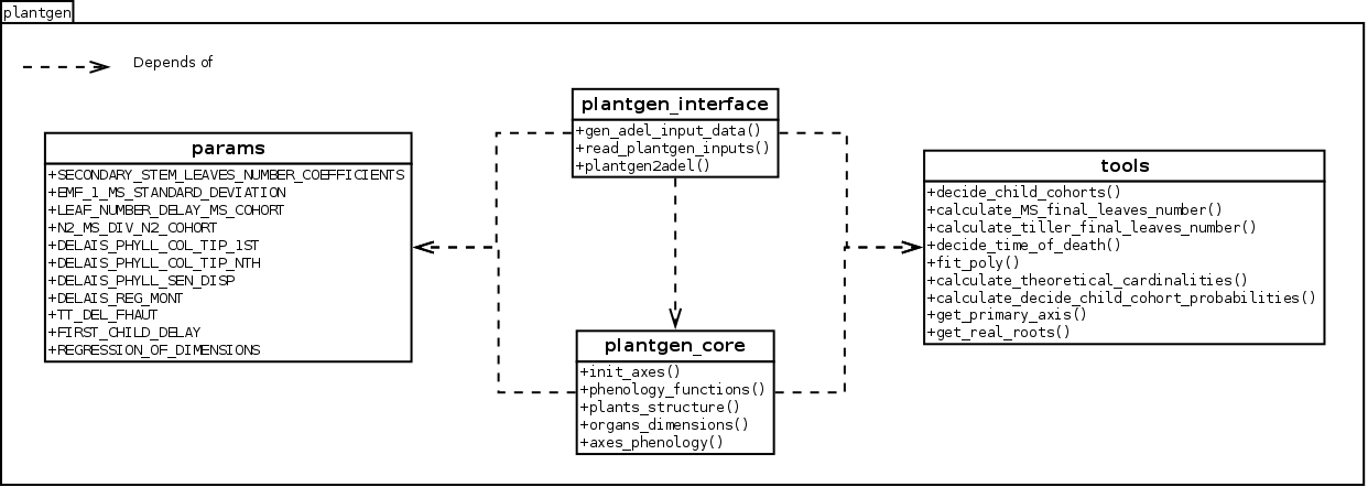
The plantgen package allows the user who does not have
a complete set of data to estimate the missing inputs.
Inside this package, the module plantgen_interface is
the front-end for the generation of the tables axeT, dimT
and phenT. plantgen_interface
also permits to generate some other tables for debugging purpose.
To construct axeT, dimT, phenT and the debugging
tables, the module plantgen_interface
uses the modules plantgen_core,
tools and module params.
The diagram static view describes the dependencies
between the different modules of the package plantgen.
We have considered three possible levels of completeness of data, denoted as MIN,
SHORT, and FULL. In the next subsections, we:
describe the levels of completeness of the data and of the parameters set
by the user,
describe how to construct the inputs of ADEL from a Python interpreter,
using the routine gen_adel_input_data.
This routine can be used whatever the level of completeness of the raw inputs,
adapting the processing automatically,
describe how to construct the inputs of ADEL from the Visualea interface,
using the node plantgen.
cardinalityT: the theoretical and the simulated
cardinalities of each cohort and each axis.
gen_adel_input_data
also produces a dictionary which stores the values of the arguments of
gen_adel_input_data.
This dictionary is aimed to log the configuration used for the construction.
The information needed to generate Adel input must be provided in two tables:
dynT_user and dimT_user. dynT_user and dimT_user can have
different levels of completeness: FULL, SHORT and MIN.
According to their level of completeness, dynT_user and dimT_user
take different shapes and/or contents.
The table below list the specific designation in plantgen
for dynT_user and dimT_user for each level of completeness:
Level of completeness
Description
dynT_user
dimT_user
FULL
the table contains data for
at least each most frequent
non-regressive axis.
First we explain the arguments of gen_adel_input_data
that the user has to define. Second we present a complete code example to use
gen_adel_input_data
from a Python interpreter.
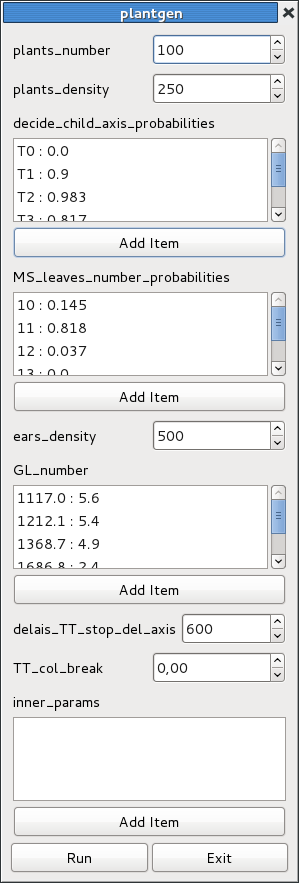
dynT_user: the leaf dynamic parameters set by the user,
dimT_user: the dimensions of the axes set by the user,
plants_number: the number of plants to be generated,
plants_density: the number of plants that are present
after loss due to bad emergence, early death…, per square meter,
decide_child_axis_probabilities: the probability of emergence of an axis
when the parent axis is present. decide_child_axis_probabilities are set
only for axes belonging to primaries tillers.
MS_leaves_number_probabilities: the probability distribution
of the final number of main stem leaves,
ears_density: the number of ears per square meter,
GL_number: the thermal times of GL measurements and corresponding values of green leaves number,
delais_TT_stop_del_axis: the thermal time between an axis stop growing and its disappearance,
TT_hs_break: the thermal time when the rate of progress Haun Stage vs thermal time is changing.
If phyllochron is constant, then TT_hs_break is 0.0.
gen_adel_input_data
checks automatically the validity of these arguments, EXCEPT for inner_params.
Thus, the user should be sure of what he is doing when setting the inner_params.
only dynT_user and dimT_user are mandatory. For all other arguments, default
value is used if no value is passed by the user.
Now let’s see a complete code example to use
gen_adel_input_data
from a Python interpreter:
# import the pandas library. In this example, pandas is used to read and# write the tables.importpandas# read the dynT_user_MIN table. "dynT_user_MIN.csv" must be in the working directory.dynT_user=pandas.read_csv('dynT_user_MIN.csv')# read the dimT_user_MIN table. "dimT_user_MIN.csv" must be in the working directory.dimT_user=pandas.read_csv('dimT_user_MIN.csv')# define the other argumentsplants_number=100plants_density=250decide_child_axis_probabilities={'T0':0.0,'T1':0.900,'T2':0.983,'T3':0.817,'T4':0.117}MS_leaves_number_probabilities={'10':0.145,'11':0.818,'12':0.037,'13':0.0,'14':0.0}ears_density=500GL_number={1117.0:5.6,1212.1:5.4,1368.7:4.9,1686.8:2.4,1880.0:0.0}delais_TT_stop_del_axis=600TT_hs_break=0.0inner_params={'DELAIS_PHYLL_COL_TIP_1ST':1.0,'DELAIS_PHYLL_COL_TIP_NTH':1.6}# launch the constructionfromopenalea.adel.plantgen.plantgen_interfaceimportgen_adel_input_data(axeT,dimT,phenT,phenT_abs,dimT_abs,dynT,phenT_first,HS_GL_SSI_T,tilleringT,cardinalityT,config)=gen_adel_input_data(dynT_user,dimT_user,plants_number,plants_density,decide_child_axis_probabilities,MS_leaves_number_probabilities,ears_density,GL_number,delais_TT_stop_del_axis,TT_hs_break,inner_params)# write axeT, dimT and phenT to csv files in the working directory, replacing# missing values by 'NA' and ignoring the indexes (the indexes are the labels of# the lines).axeT.to_csv('axeT.csv',na_rep='NA',index=False)dimT.to_csv('dimT.csv',na_rep='NA',index=False)phenT.to_csv('phenT.csv',na_rep='NA',index=False)# "axeT.csv", "dimT.csv" and "phenT.csv" are now ready to be used by Adel.
fromopenalea.adel.plantgen.plantgen_interfaceimportread_plantgen_inputs# "plantgen_inputs_MIN.py" must be in the working directory(dynT_user,dimT_user,plants_number,plants_density,decide_child_axis_probabilities,MS_leaves_number_probabilities,ears_density,GL_number,delais_TT_stop_del_axis,TT_hs_break,inner_params)=read_plantgen_inputs('plantgen_inputs_MIN.py')# launch the constructionfromopenalea.adel.plantgen.plantgen_interfaceimportgen_adel_input_data(axeT,dimT,phenT,phenT_abs,dimT_abs,dynT,phenT_first,HS_GL_SSI_T,tilleringT,cardinalityT,config)=gen_adel_input_data(dynT_user,dimT_user,plants_number,plants_density,decide_child_axis_probabilities,MS_leaves_number_probabilities,ears_density,GL_number,delais_TT_stop_del_axis,TT_hs_break,inner_params)# write axeT, dimT and phenT to csv files in the working directory, replacing# missing values by 'NA' and ignoring the indexes (the indexes are the labels of# the lines).axeT.to_csv('axeT.csv',na_rep='NA',index=False)dimT.to_csv('dimT.csv',na_rep='NA',index=False)phenT.to_csv('phenT.csv',na_rep='NA',index=False)# "axeT.csv", "dimT.csv" and "phenT.csv" are now ready to be used by Adel.
read_plantgen_inputs
permits the user to store the arguments, so he can reuse them later.
plantgen is located in openalea.adel.plantgen.
You can access to plantgen through the package explorer of VisuAlea,
or just typing “plantgen” in the Search tab of VisuAlea.
The associated widget, which appears when you open plantgen, permits to
configure the construction.
The user must select existing data nodes to set the input and ouput tables.
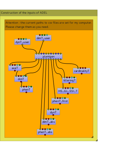
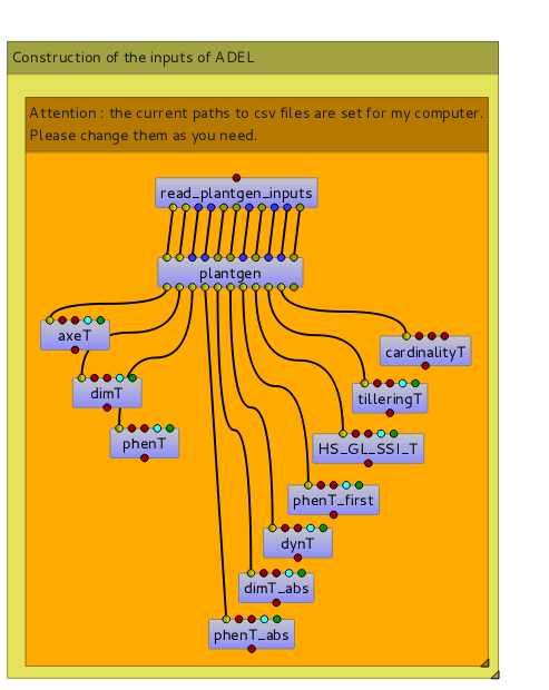
The following data-flow demonstrates another way to use plantgen through
Visualea:
The openalea.adel.Tutorials.plantgen_csv dataflow#
In this case the user must give the paths of csv files for inputs and outputs.
Warning
the paths set in openalea.adel.Tutorials.plantgen_csv will not work
on your computer. You have to adapt them to your needs.
Finally, the node read_plantgen_inputs permits to define the values of the input ports of
plantgen by importing a Python module. read_plantgen_inputs is also located in
openalea.adel.plantgen.
For example, using read_plantgen_inputs with the module
plantgen_inputs.py,
the dataflow becomes:
The openalea.adel.Tutorials.plantgen_csv_inputs dataflow#
read_plantgen_inputs permits the user to store the values of the input ports,
so he can reuse them later.
SECONDARY_STEM_LEAVES_NUMBER_COEFFICIENTS:
the coefficients a_1 and a_2 to calculate the final number of leaves on tillers from the final number of leaves on main stem.
EMF_1_MS_STANDARD_DEVIATION:
the standard deviation in the thermal of emergence of plants in the plot.
LEAF_NUMBER_DELAY_MS_COHORT:
the delays between the emergence of the main stem and the emergence of each cohort.
N2_MS_DIV_N2_COHORT:
ratio between the maximum number of green leaves on the tillers and the maximum green leaves on the main stem
DELAIS_PHYLL_COL_TIP_1ST:
delay between tip appearance and collar appearance for the first leaf only.
DELAIS_PHYLL_COL_TIP_NTH:
delay between tip appearance and collar appearance for all leaves except the first one.
DELAIS_PHYLL_SEN_DISP:
the time during which a fully senesced leaf on a non-elongated internode remains on the plant.
DELAIS_REG_MONT:
the time between the start of the regression and the start of MS elongation.
TT_DEL_FHAUT:
the thermal time at which leaves on elongated internode disappear.
FIRST_CHILD_DELAY:
the delay between a parent cohort and its first possible child cohort
REGRESSION_OF_DIMENSIONS:
the regression of the dimensions for the last 3 phytomers of each organ.
These parameters can be set by the user through the input argument inner_parameters
of the function gen_adel_input_data, or
set directly in the module params.
They permit a finer parameterization of the construction.
The function RunAdel permits to simulate 3D architectural
development of the shoots of wheat plants, according to a list of dates (thermal times) and
Adel’s inputs (see Description of Adel’s inputs).
RunAdel returns a Python dictionary. Each key
of the dictionary represents an output.
The following table describes each of these outputs.
Output of RunAdel
Description
refplant_id
plant id
axe_id
axe id
ms_insertion
phytomer insertion position, starting from the base (not normalized)
nff
final number of leaves produced by the axe
HS_final
final haun stage reached by the axe (determine regression or not)
numphy
phytomer position (from bottom)
ntop
phytomer position (from top)
L_shape
lamina length (cm)
Lw_shape
lamina width (cm)
LsenShrink
shrink in lamina width due to senescense. Width is the remaining width proportional to the blade width before senecened
LcType
selector for first level in leaf database (ntop). First level is the leaf type indexed by the phytomer position (ntop).
LcIndex
index for selecting the leaf geometry from the replicates of the same phytomer (LcType)
Linc
inclination of the base of the lamina relatively to the sheath (deg)
Laz
azimuth relative to the previous leaf ( Laz[1] = azT, Laz[2:end] = azim) (azT refers to the the azimuth(deg) of the first leaf of the axis with reference to the azimuth of the parent axe. azim refers to the azimuth (deg) of the leaf compared to the previous one. azT and azim are defined in the user-defined function, geoAxe and geoLeaf, respectively.)
Lpo
proportion of green tissue in the lamina (on a length basis)
Lpos
proportion of senescent tissue in the lamina (on a length basis)
Gd
apparent diameter of the sheath
Ginc
inclination relative to of the previous sheath
Gpo
proportion of green tissue in the sheath (on a length basis)
Gpos
proportion of senescent tissue in the sheath (on a length basis)
Ed
diameter of the internode in cm
Einc
inclination relative to of the previous internode
Epo
proportion of green tissue in the internode (on a length basis)
Epos
proportion of senescent tissue in the internode (on a length basis)
rph
normalized phytomer position (= numphy/nff ) ?? to be confirmed
rssi
relative senescence index (ssi - numphy)
rhs
relative haun stage (haun stage - numphy)
Then, the function mtg_factory permits to
construct a MTG from the output of RunAdel.
The appendices describe the data used by Adel for pre and post-processing.
The appendices also contains static and dynamic view of the system, to
help the user understanding hwo it works.
Then, we describe the data used in the construction of the input tables of Adel:
dynT_user_FULL: the dynamic of the Haun stage of
at least the most frequent non-regressive axes.
dynT_user_SHORT: for each id_axis, the dynamic of the
Haun stage of exactly the most frequent non-regressive axes.
dynT_user_MIN: the dynamic of the Haun stage of
the most frequent main stem, and, for each primary axis, the thermal time when
Haun Stage is equal to the final number of phytomers.
dimT_user_FULL: the dimensions of
at least the most frequent non-regressive axes.
dimT_user_SHORT: the dimensions of
exactly the most frequent non-regressive axes.
dimT_user_MIN: the dimensions of the most frequent
main stem.
phenT_abs: the equivalent of phenT, but
with absolute thermal times and absolute phytomer ranks.
dimT_abs: the equivalent of dimT, but with
absolute phytomer ranks.
dynT: the dynamic of the Haun stage for each axis.
phenT_first: a subset of phenT_abs,
containing only the lines of phenT_abs which correspond to the first
phytomer of each cohort.
HS_GL_SSI_T: the dynamic of Haun stage, green leaves and
senescent leaves when thermal time varies, for each cohort.
dynT_user_FULL is a table which describes the dynamic of the Haun stage of
at least the most frequent non-regressive axes. The most frequent axes are
the axes which have the most frequent number of phytomers.
dynT_user_FULL contains a line of data for at least each couple (id_axis, most frequent N_phytomer_potential),
where id_axis and N_phytomer_potential are defined in axeT.
Each line contains the following data: id_axis, N_phytomer_potential, a_cohort,
TT_hs_0, TT_flag_ligulation, n0, n1 and n2.
See dynT for the meaning of these parameters.
dynT_user_SHORT is a table which describes the dynamic of the Haun stage of
exactly the most frequent non-regressive axes. The most frequent axes are
the axes which have the most frequent number of phytomers.
dynT_user_SHORT contains a line of data for exactly each couple (id_axis, most frequent N_phytomer_potential),
where id_axis and N_phytomer_potential are defined in axeT. The couples (id_axis, NOT most frequent N_phytomer_potential)
are not documented in dynT_user_SHORT.
Each line contains the following data id_axis, a_cohort, TT_hs_0,
TT_flag_ligulation, n0, n1 and n2.
See dynT for a description of these parameters.
dynT_user_MIN is a table which describes the dynamic of the Haun stage of
the most frequent main stem. The most frequent main stem is the
main stem which has the most frequent number of phytomers.
dynT_user_MIN also contains, for each primary axis,
the thermal time when Haun Stage is equal to the final number of phytomers.
The first line contains the following data: id_axis, a_cohort, TT_hs_0,
TT_flag_ligulation, n0, n1 and n2.
In the other lines, only id_axis and TT_flag_ligulation are documented:
a_cohort, TT_hs_0, n0, n1 and n2 are NA (i.e. Not Available).
dimT_user_FULL is a table which documents the dimensions of
at least the most frequent non-regressive axes. The most frequent axes are
the axes which have the most frequent number of phytomers.
dimT_user_FULL contains a line of data for at least each couple (id_axis, most frequent N_phytomer_potential),
where id_axis and N_phytomer_potential are defined in axeT.
Each line contains the following data: id_axis,
N_phytomer_potential, index_phytomer, L_blade, W_blade, L_sheath, W_sheath,
L_internode and W_internode. id_axis are the botanical positions (see
Botanical position of the axis on the plant.). N_phytomer_potential are the final number of phytomers. The
other data are the same as the ones in dimT_abs.
dimT_user_SHORT is a table which documents the dimensions of
exactly the most frequent non-regressive axes. The most frequent axes are
the axes which have the most frequent number of phytomers.
dimT_user_SHORT contains a line of data for exactly each couple (id_axis, most frequent N_phytomer_potential),
where id_axis and N_phytomer_potential are defined in axeT. The couples (id_axis, NOT most frequent N_phytomer_potential)
are not documented in dimT_user_SHORT.
Each line contains the following data: id_axis, index_phytomer, L_blade, W_blade, L_sheath, W_sheath,
L_internode and W_internode. id_axis are the botanical positions (see
Botanical position of the axis on the plant.). N_phytomer_potential are the final number of phytomers. The
other data are the same as the ones in dimT_abs.
dimT_user_MIN is a table which documents the dimensions of each phytomer of
the most frequent main stem. The most frequent main stem is the
main stem which has the most frequent number of phytomers.
Each line contains the following data: index_phytomer, L_blade, W_blade,
L_sheath, W_sheath, L_internode and W_internode.
See dimT_abs for a description of these data.
phenT_abs is an intermediate table used to construct phenT.
This table is not an input of Adel. Thus the user normally needn’t it. This table
can be useful for debugging.
dimT_abs is an intermediate table used to construct dimT.
This table is not an input of Adel. Thus the user normally needn’t it. This table
can be useful for debugging.
dimT_abs is the same as dimT, except that the positions
of the phytomers are not normalized.
dynT is an intermediate table used to construct the input of Adel.
This table is not an input of Adel. Thus the user normally needn’t it. This table
can be useful for debugging.
dynT is a table which describes the dynamic of the Haun stage of
all non-regressive axes.
For each couple (id_axis, N_phytomer_potential) in axeT, dynT contains
a line with the following data:
phenT_first is an intermediate table used to construct phenT and
axeT. This table is not an input of Adel. Thus the user normally
needn’t it. This table can be useful for debugging.
phenT_first is a subset of phenT_abs, and contains only the lines of
phenT_abs which correspond to the first phytomer of each non-regressive axis,
i.e. index_phytomer equal to 1.
tilleringT describes the dynamic of tillering. It stores the number of axes
per square meter at important thermal times: the start of growth, the thermal time
of the start of MS elongation, and the thermal time of the flowering.
cardinalityT is constructed for debugging purpose.
cardinalityT describes the theoretical and the simulated cardinalities of
each cohort and each axis. It permits the user to validate the simulated cardinalities
against the theoretical ones.
Both cardinalities are calculated from the probabilities of emergence of an axis
when the parent axis is present. These probabilities are given by the user.
Theoretical cardinalities are calculated globally without randomness.


 ;
Senescence of each upper leaf blade progresses first at a slow rate,identical for all leaves, then at a fast rate.
;
Senescence of each upper leaf blade progresses first at a slow rate,identical for all leaves, then at a fast rate.